Abstract
“Face Recognition” – this is this year’s topic of the master practical course “Application Challenges for Machine Learning on IBM Power Architecture”. As this topic is already well researched, we spent our first efforts on getting an overview of the current state of the art. The conclusion of that investigation was that Siamese Neural Networks seem to be the most appropriate solution for that scope of application. Despite using a Nvidia xyz CPU the computing power still is a finite resource. To overcome this bottleneck, we decided to use Transfer-Learning and used different pretrained neural networks. To make the training harder and hence improve the accuracy of our models, we decided to implement a two-stage triplet-selection. The underlying idea is, that the negative images of the triplets have a strong similarity to the positives and the anchor, so that the neural network is learning the features with the most informational value.
We implemented a transfer learning approach that combines densenet161 for facial feature extraction and additional layers for an optimal image embedding. This model architecture achieved a validation accuracy of more than 99.5%. After having learnt to embed images, the model’s inference is used to perform one-shot-learning. In one-shot-learning, an unseen image of a new person is embedded and added as an additional anchor. Given another unseen image of this person the system then can correctly associate the person on the image with the newly learnt anchor. As this is done after having only seen one anchor image, this is called one-shot-learning.
Team
Team Members
Our team consists of four members out of the study programs “M.Sc. Robotics, Cognition, Intelligence”, “Postgraduate studies in Informatics”, “Information Systems”, and “M.Sc. Informatics”.
 Benjamin Betz, 24: M.Sc. Informatics, Data & Preprocessing Guru |  Sami Ibishi, 29: M.Sc. Robotics, Cognition, Intelligence, Deep Learning Guru |
 Manuel Styrsky, 23: M. Sc. Information Systems, Hyperparameter Tuning Guru |  Michael Hussak, 27: Postgraduate Studies in Informatics, Data Scientist & Frontend Expert |
Project Organization
To maintain an overview of the project, the team was organized in accordance to the SCRUM methodology and used Meistertask as SCRUM board:
- Weekly sprints via Zoom
- Define and distribute tasks together as a team and assign to one team member to have clear responsibilities
- Frequent arrangement meetings in sub-teams
- Clear communication of final decisions
For more advanced topics we often worked together as a team and did Pair- and Mob-Programming. Doing this helped each team member to understand the underlying code and to avoid and prevent coding errors (syntax errors as well as logic errors).
To bear the coding progress of other team members in mind and to ensure good code quality, a code review process was installed. This review process is based on the dual control principle: To merge one’s changes into the main branch of our repository, somebody else needs to review these changes and approve them.
Project Plan
The Gantt-Chart in Figure 1 is based on the timeline presented in the intermediate presentation. Additionally, we added the idea of using Streamlit to showcase our model in use.
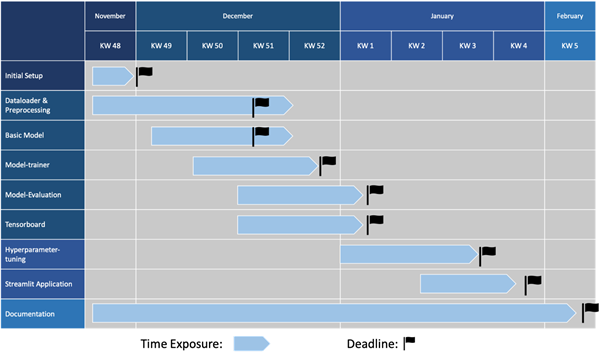
Figure 1: Gantt-Chart of the Face Recognition Project
Except for the working packages ‘Dataloader & Preprocessing’ and ‘Basic Model’ we have been well within the timetable. As the technical integration to Streamlit has been straightforward, we finished it ahead of our schedule.
The delay in Dataloader & Preprocessing can be explained by introducing new ideas and meeting upcoming requirements. As most of these ideas came up during testing, we had to modify retroactively.
To set up a basic model, it took more time than expected to compose the various code components. The challenging task in this case was to adjust the interface functions to comply with the requirements.
Irrespective of the above mentioned, by using the planned buffer time we were able to finish the project in time and fulfill our set goals.
Project Topic and Motivation
Project Topic
The topic of our project was to build a neural network for face recognition. Currently, there exist already various fields of applications for face recognition. It is used to grant access in diverse scenarios (e.g. to unlock a smartphone or to enter a building) as well as to perform an identity check (e.g. for banking applications).
As we got the freedom to evolve the project in any direction, we decided to set the focus on an optimized model instead of building a framework or an application around a model. As all team members were willing to extend their skills, we decided to use the PyTorch library instead of Tensorflow. A careful inspection of the current state of the art papers led us on the track of Siamese Neural Networks. In the course of time, we explored various possible improvements that resulted in the neural network described in the following.
Motivation, State of the Art and Model
To gain an overview of the topic of face recognition, we started the project with a scientific investigation. This helped us understanding the structure and methods used in state of the art models as well as identifying the challenges of current research projects.
The origins of face recognition go back to the 1990s and 2000s and started with holistic approaches. Those approaches based on extracting low dimensional characteristics by distribution assumptions [1]. In the following, shallow methods were the primary interest of research. In the process of time, it transpired that these shallow methods do not lead to sufficient and stable performance, as they are not able to extract different facial invariants at a time. The breakthrough in face recognition was achieved in 2012and in 2014 respectively by using deep learning. Deep learning boosted the accuracy up to 97.35% [2] which is comparable to a humanly possible accuracy (97.5%). Since then, the focus of research has been on deep-learning based approaches and, as well as different algorithm designs, datasets and evaluation protocols [1].
The current areas of research in the domain of face recognition can be split amongst the following criteria:
- Loss function: As softmax loss is widely used in object recognition, attempts are made to also use it in face recognition. Different variations of softmax are trying to use normalized features and weights to improve performance. However, lacking the ability to learn more discriminative features, new loss functions are being explored [1]. Reasonable approaches are based on Euclidean loss functions, e.g. contrastive loss and triplet loss. The contrastive loss is optimizing by distance between two images. The two images are converged in case they depict the same person and are separated if they show different ones. Triplet loss is using three different images, an anchor image, a positive and a negative image. The goal of triplet loss is to minimize the distance between anchor and positive and maximize the distance between anchor and negative [3][4].
Other approaches are based on angular/cosin-margin. In case they are used with a clean dataset, they are able to achieve good results. However, they are very vulnerable to noise.
Based on that, we decided to use a triplet loss in our project implementation. - Network architecture: During the research phase, it became clear that the current state of the art works are all based on a choice of architectures. These include AlexNet, ResNet, VGG16 and VGG19 [5] as well as GoogleNet [1]. Therefore, we resolved to apply transfer learning, by basing our model on the aforementioned networks and then extending them by various layers.
- Data based differences: One of the greatest factors of uncertainty in face recognition is constituted by the input data. There exist various research projects about the topic of handling noisy data. Many algorithms for example are struggling to correctly identify images in profile view[6]. To face this issue, attempts are made to reconstruct a frontal view out of profile views of different angles. Another challenging topic in face recognition is aging. As the facial appearance changes over time, it is extremely challenging for a neural network to learn certain features. Currently, there are two main strategies to overcome this problem:
- Reconstruct an image to a target age and perform the face recognition on the same age group [1]
- Put stronger emphasis on age-independent features[7]
For the sake of completeness, it should also be
mentioned that images of heavily made-up persons might be challenging to learn,
as distinguishing features may be hidden [8].
Besides these person-based factors, the photographic quality of an image also plays
an important role. Bad lighting and exposure errors, as well as a low
resolution need to be treated in a special manner, to not distort the network
while training.
The central issue of face recognition in industry is to make it robust against attacks. As spoofing current systems is still possible, companies have legitimate concerns about deploying face recognition systems in safety-critical areas. The most promising strategy is the use of 3D face recognition. However, due to the difficult acquirement of 3D faces and limited publicly available datasets, research is still in its infancy.
Based on the above mentioned, we decided to build a widely usable network and thus not focus solely on pose, age, or any other specialization. Our dataset contains all varieties of facial representations and different qualities.
Face Recognition
ML Approach
Face recognition is a technique that has the objective to recognize and identify a person based on their facial features. To accomplish this, a system takes a new image of the person to be identified and compares this visual information with stored images of all known people. This comparison is implemented through a similarity function. The similarity function can be formulated in various ways. However, they all have one core idea in common: They calculate a value that resembles how much of the facial information in both images overlap. A person is recognized, if the similarity between the new image and one of the stored images is smaller than a predefined threshold.
Many different approaches tackle the challenges of face recognition. Classical computer vision and traditional machine learning approaches used hand-picked or statistically gained filters to extract features, recognize patterns or find facial landmarks. The performance achieved with those techniques under certain constraints on the lighting, the face position, the facial expression, as well as other factors, were good. Although they could not reach human-level performance. The progress made with those techniques was in general slow and narrow. The research mostly focused on solving specific issues like different lighting or different facial expressions [9] [10] [11].
Since the uprise of deep learning techniques, especially the achievements of deep learning methods in the ImageNet competition, the research of face recognition started to focus on neural networks. Deep learning approaches started to improve the generalization of the algorithm and increased the overall performance of face recognition. One such example is DeepFace, which was proposed in 2014. It was the first human-level face recognition approach without any constraints on the test environment or test data [12]. Many other approaches followed DeepFace, like FaceNet [13], VGGFace [14], VGGFace2 [15]; which pushed the performance even beyond human-level performance. Based on those results we decided to implement our face recognition in a common deep learning fashion, like FaceNet [13].
Model Input Data
The given inputs are regular RGB images with pixel values from 0 to 255. All images in the dataset we use contain cropped and centered faces. Therefore, our model does not need to detect one or even multiple faces first. It only needs to learn to identify the person in every image.
The shape of one image is defined as follows, shape = [ Width, Height, Channel]. The channel dimension represents the three primary colors. The width and height dimension renders the spatial size of the seen image. Our model needs to fulfill many conditions. One of them is that it should handle different input sizes in the test phase. The input size refers here only to the width and height dimension. In the training phase, we will only use images of size 224x224 because of performance and memory reasons. Those are the most important technical details about the input data. Further information regarding a more in-depth exploration of the input data can be found in the section: The Dataset.

Model Output
The goal of the model is to create a reasonable vector representation of every face (image). In other words, a unique numerical embedding of all facial information can be used to identify a specific person. Furthermore, this embedding process should be able to embed new and different images of the same person in proximity based on a certain metric. Such that a similarity value can be assigned between the original and the new input. Those metrics can be implemented in various ways, such as the distance or the angle between two embedding vectors. This mostly depends on the design decision. Since we decided to go for the FaceNet architecture, we will use the Euclidean distances between the embedded images as a similarity value, to stay close to the original proposal.
One more design decision we had to make regarding the output of the model was the size of the embedding vector. A very large vector implies a large hyperspace which allows the model to embed images very sparse and distributed. That would make the training process quite easy, since the distances would instantly be chosen relatively large. But this would use a lot of memory unnecessarily and make the whole model larger than it needs to be. Furthermore, we could end up overfitting the model such that only the same image could be used to identify the person. Therefore, we decided to start with a small embedding size and then progressively increase it based on the performance and the amount of data (number of person/ids) we used for training.
FaceNet Architecture
As already explained in section ML Approach, we were inspired by the FaceNet [13] concept. They used a series of convolutional layers and one fully connected layer to extract all relevant features. Followed by a normalization layer, which uses the L2 norm to normalize the extracted feature vector into the embedding vector. The purpose of the normalization is to constrain the embeddings on the hypersphere with a radius of 1. The concept of the FaceNet architecture is pictured in the following figure:
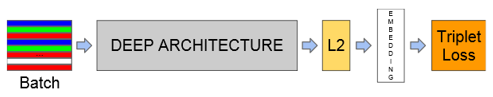
In the FaceNet paper, they proposed different deep architectures to extract the facial features. Using different concepts to leverage the convolutional neural networks to the fullest. One approach was to use multiple inception layers. Since we had limited computational power and we used a smaller dataset than the authors of FaceNet, we decided to only extract the core ideas of their proposal.
Features and Functionality
To fulfill the imposed requirements and due to the limitation in time, our features are separated in Must-Haves and Nice-to-Haves. The Must-Haves were given by the conceptual formulation and represent some basic features of face recognition. Unlike the Must-Haves, we were entrusted to extend the task by self-defined Nice-to-Haves. These Nice-to-Haves are additive; thus, they had a lower priority and were implemented depending on the remaining time.
In the following section we provide an overview of how we interpreted those requirements and how we implemented them, including some graphical illustrations.
Must-Haves
General Functionality
A given assumption was that the input images only portray one person and are using the RGB color space. The images of our dataset visualize the person in portrait in such a manner that they were cut at shoulder level. Therefore, preprocessing, such as first detecting the face and then extracting it, was redundant.
In the course of the project, it became apparent that using a pretrained neural network is a reasonable approach. To get the greatest benefit out of the pretrained model, we reshaped the input images in conformity to the input dimensions of these models. Therefore, another hard requirement could be met. More details about the exact implementation will be explained in the ongoing chapters and can also be seen in examined in the Github-Repository.
One-Shot-Learning
One-Shot-Learning is a highly topical area of research. As the name suggests, One-Shot-Learning is a method which enables a neural network to learn given only a single training example. In practice, this application works as follows: After adding a single new image of a person (so called anchor image) to the set of known persons, other unseen images of this person will be recognized and associated to the training image. Siamese Neural Networks are very well suited for this scope, as they are trained to measure the distance between two input images. The first step is to calculate the embedding of the anchor image. In the second step, the embeddings of other unseen images will be calculated. By calculating the distance between those images and the anchor image and by using a threshold, it can be distinguished if the person on the image is the same as the one displayed in the anchor image or not.
To illustrate this, we decided to use the framework streamlit. The application can be started by:
streamlit run /path/to/streamlit_script.py
By switching the app mode to ‘One Shot Learning’, a pretrained model is loaded in the background and the user is ready to go. In the first step, the user needs to add a new Person as anchor to the database. This can be done by uploading a new anchor image and defining its ID. As soon as both inputs are entered, this person is added to the database and its embedding is calculated.

Now the image will be displayed, and the user is ready to perform the second step. In this step, the user has to enter a relative path to a directory containing multiple test images. This folder with test images may contain multiple, one or no image of the person with the ID selected in step 1.
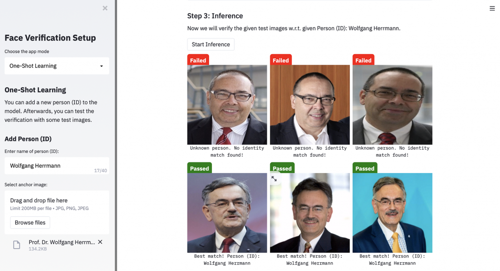
The last step of this demo is the inference. By pressing the ‘Start Inference’ button, the distances between all test images and the anchor image will be calculated and compared with the defined threshold. The result of the inference is displayed above every test image. In case the test image matches with the uploaded anchor image, its ID will be displayed as a subtitle below the image.
Nice-to-Haves
Besides the Must-Haves, we agreed on various Nice-to-Haves. After defining them, we prioritized these features and implemented them depending on time. They are listed in descending relevance below:
- Tensorboard
- Handle different input image formats
- Handle images with multiple persons
- If person not recognized: option to directly add to Known-Person-Dataset
- Aggregate verification attempts per unknown person
During the project, we focused on the best possible performance of our neural network. This is the reason why the last three Nice-to-Haves were not implemented. To visualize the model and to be able to track the training progress, we decided to use tensorboard. In fact, most of the plots and visualization, of our model and the training, across this documentation were extracted from tensorboard.
The Dataset
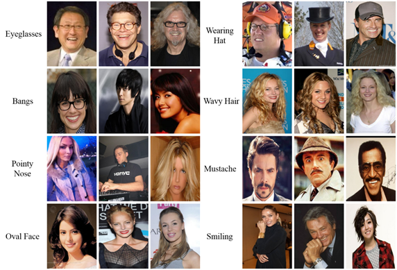
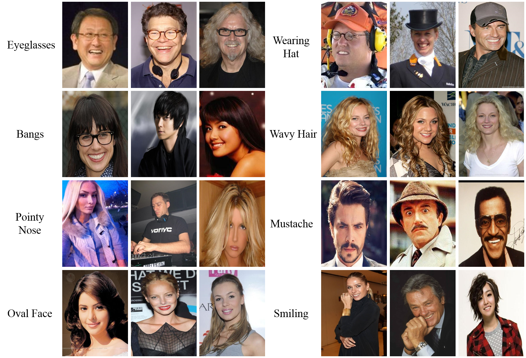
To train our model we used a subset of the Large-scale CelebFaces Attributes (CelebA) dataset as an extensive source of face images. CelebA is part of the paper “Deep Learning Face Attributes in the Wild” [16]. It consists of about 200,000 annotated images of celebrities that were cropped around the face of the respective person. For our subset, we selected the first 10,000 images out of this dataset.
We chose this dataset to train our model because it provides the following advantages:
| Dataset property | Examples | Advantage for our model |
| Large pose variations | Frontal/profile view Low/high angle | Model can learn a more general representation of the face |
| Obscured faces | Sunglasses, hats | Learn to represent faces with missing features |
| Background clutter | Colored background Other faces in image | Model needs to focus on the face and ignore background noise |
| Large diversity | Gender, age, ethnicity | Learn diverse faces & use diverse negatives to train against |
| Large quantity | Many image samples per celebrity | Multiple positives to train the triplet network on |
Downloading and Preprocessing
The first step of using a dataset
of course always is to get your hands on it. Thus, prior to data preprocessing
and using it for our model, we first automated this tedious step.
Including several options such as destiny file location or whether to unzip the
file, our downloading functionality takes care of this. Utilizing the gdown package to easily obtain openly
accessible google drive files, we first download the entire zipped dataset.
Then, we proceed to unzip the dataset and perform a basic, yet crucial
preprocessing step on it:
With the help of the label file, which is a dict-like text file containing
pairs of image IDs and their associated labels for all images, we create a new
directory structure. We group each image of the same person (same ID) into the
same directory. This structure proved important, as it significantly simplifies
the subsequent process: the triplet creation. Another parameter that comes into
play at this point of structuring the dataset, is the minimum number of positives. It defines which IDs will be kept in
this preprocessing step: If a person does not appear sufficiently often in the
dataset, we discard all respective images of that particular person. As part of
hyperparameter tuning, having 5 samples available per person emerged as a fine
choice.
Triplet creation
After having performed the above preprocessing steps on the dataset, we can now proceed to further tailor it to fit our Siamese Neural Network architecture. The requirement is to prepare the images in a fashion that yields a triplet of:
Anchor: Reference image of a person
Positive: Image of the same person as the anchor, but not the anchor itself
Negative: Image of a different person
For each combination of anchor and positive we used five different negatives, such that the model can really learn the facial features by distinguishing them among a large quantity of adversarial examples. At the beginning of the course of the project, the triplet creation was completely randomized.
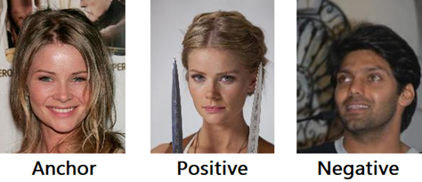
The only two basic requirements
fulfilled by this first approach were that the anchor and the positive were not
identical and that the negative showed a different celebrity than anchor and positive.
This also meant that the anchor could potentially depict the person’s face in a
(partially) concealed manner – for example wearing a hat and sunglasses – or at
an uncommon angle or head tilt. But the model would always consider this
imperfect image as the best reference of the person. Additionally, the randomly
chosen negative could be entirely different, which can be observed in the above
illustration. This is not ideal, as the model barely has any effort to move the
embeddings of the images away from each other, because they already inherently
differ. Thus, the model barely learns anything from this triplet.
During the project, a more sophisticated approach to this data preparation step
was deemed necessary to avoid creating these ‘useless’ triplets and to further
improve the performance of our model. Thus, we introduced more requirements on
the selection of the anchor and the negatives which will be described in the
following paragraphs.
Choice of Anchor Images
To choose the best possible anchor image among all samples of a given person, we consider a vector representation of all these samples. We achieve this representation by utilizing the model densenet161 of the torchvision library. By stopping the inference of the densenet161 model at the third last layer, we obtain a large (size 1024) Tensor for each image. Then we can compute the mean out of all these Tensors, thereby ‘averaging’ the image samples of this person. Using the L2 loss, we now deduce which image is the closest to this mean representation, thus yielding our anchor.
Choice of Negatives
With a similar approach we also enhanced our selection of negatives for each pair of anchor and positive: Again, using the L2 loss on the image vector representations, we choose the negative to be of minimal distance to the positive. This increases the difficulty of the model’s learning process, as now we really force the model to push the image embedding of the positive closer to the anchor.
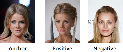
The model now cannot just use the entire vector space to its full extent, in order to sufficiently separate the embeddings. The model’s previous, lazy behavior of choosing embeddings such that they barely undercut the threshold for a correct classification is thus made more difficult.
Image Resizing and Train-Validation-Split
The final necessary steps are to prepare
these triplets to be processable by the model.
We divide the entire dataset into a Training Subset and a Validation Subset
with a basic 90/10 train/val split. Different splits we tried were 70/30 and 80/20
but they did not lead to any improvements, thus we adhered to the 90/10 split.
Additionally, when the _getitem_ method
of our dataloader is called, we first resize the image to compatible dimensions
for our model. As our model expects images of size 224x224 as input – and in
fact this is a common size expected by many other image processing neural
networks as well – we tailor the image to fulfill this property before
returning it.
These steps conclude the preprocessing part of our model’s pipeline.
Face Recognition - Our Approach
In the following Section we describe how we solved the problem of face recognition.
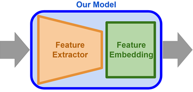
Our Model
We decided to go for a modular two-stage network. The schematic concept of this principle is visualized in the following figure. The first stage is implemented with convolutional neural networks, which focus on extracting the most important visual information, i.e., facial features. The second stage of our model utilizes the extracted features to find the optimal feature embedding to create a distinct vectorized representation of the different people (ids) from our training dataset. For this part, we leveraged the capabilities of fully connected neural networks. The idea behind the separation into those two parts is that it allows us to easily exchange one part of the network without breaking the entire system. This concept will be utilized in the optimization of our model, which will be explained in more depth in the section Hyperparameter-Tuning.
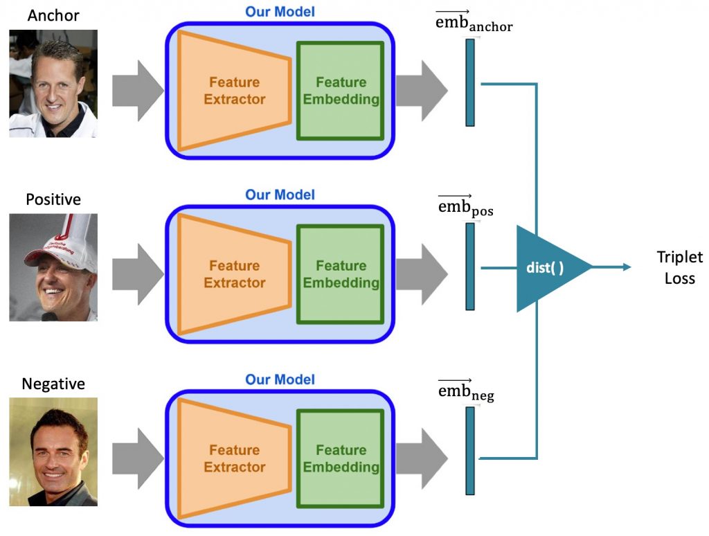
For the face recognition task, it is quite common to use the Siamese Neural Network architecture, where two models embed their inputs. The outputs of those two models are then forwarded to the distance calculation part. One of the most important details about this model architecture is that the two models share the same weights. This means, that the implementation itself can be simplified: Instead of implementing two separate models, only one model is built and trained. In this sense, the Siamese Neural Network is a more abstract architecture than a physical one. To utilize those architectures, it is necessary to always calculate two inputs consecutively to gain one prediction. Since we decided to go for a similar approach as proposed in FaceNet, we decided to go for a triplet network fashion. Which is an extended version of the Siamese Neural Network. It will take triplets (Anchor, Positive, Negative) as input and create three embedding vectors. The triplet network is visualized in the following figures.
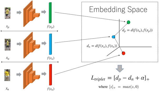
Triplet Loss Function
The criterion we used to evaluate and optimize the embedding quality is the “Triplet Loss Function”. It uses the calculated distances d(a, p) between the anchor image xia of a person (id) and all positive images xip which contain the same person (id). As well as the distances d(a, n) between the anchor image xia and all negative examples xin which contain any other person but the one in the anchor image. Those distances are then used in the triplet loss function for comparison. There, the triplet loss penalizes the embedding of the model, if the distance between anchor and negative is smaller than the distance between anchor and positive. If the distance between anchor and positive is already smaller than the distance between anchor and negative, the function returns no penalty. In order to increase the quality of the embeddings, it is common to add an additional margin α to push the negative examples further away. Regarding the distance function d(•), any distance function that maps the two input vectors to a single value representing a similarity value can be chosen. However, it is very common to use the Euclidean distance, which we also decided for [4]. The concept of the triplet loss is mathematically defined as follows:

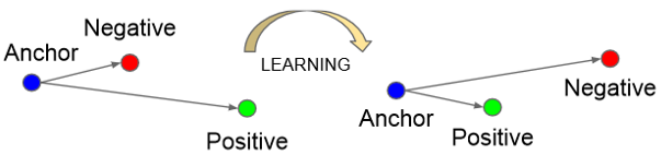
Where T includes all possible triplet combinations from the given dataset. Since many combinations would already fulfill this formulation, we normally selected only difficult triplets which is explained in chapter Downloading and preprocessing. The function f(•) represents the image embedding created through the trained model. The following figure visualizes the learning procedure.
The triplet loss function to optimize the model for its embedding purposes:

Transfer Learning
The basic idea behind transfer learning is to reuse an already pre-trained model for the current task. To leverage those models, they need to be trained on a similar task. The meaning behind a similar task in the context of machine learning is the similarity of the underlying distribution in the datasets. This can be explained in the field of computer vision quite intuitively. For example, a model trained for image classification, e.g. on the ImageNet dataset, which classifies images into more than 2000 (dog, cat, person, car, …) different classes can be reused for a specific classification, e.g. dog breed classification. The model trained for ImageNet already learned to extract and prioritize certain visual features which are important for the second task as well, since the visual features in both datasets overlap. What is common for the deep learning architecture is to take a pre-trained model as a backbone model and only adapt the last couple of layers or add new layers to fit the new task. We decided to leverage the benefits of transfer learning as well. Therefore, we searched for models that were trained on a broad field of visual inputs and had high accuracy in classification. Which lead us to pre-trained models on the ImageNet dataset. After a few investigations and testing, we decided to take a closer look at the following three pre-trained models.
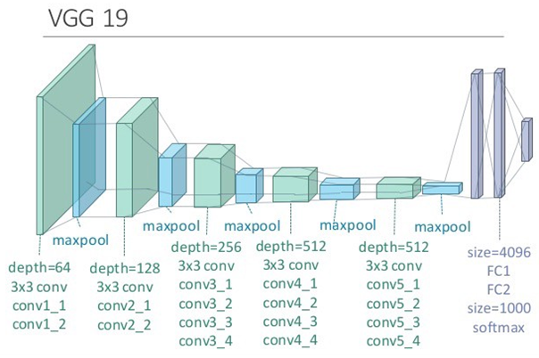
VGG19
VGG networks were proposed in Very Deep Convolutional Networks for Large-Scale Image Recognition. The authors of this paper investigated the correlation between the performance and the depth of neural networks. They showed the effectiveness of very deep neural networks on a range of different tasks. The pre-trained VGG models are a good starting point for many visual tasks. The architecture of VGG19 is pictured in the following figure:
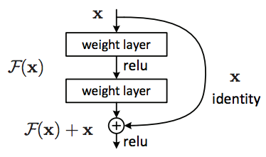
ResNet
ResNet models were proposed in “Deep Residual Learning for Image Recognition” paper. The authors of this paper investigated the difficulties to train very deep neural networks. They especially focused on the issue that the backpropagated values got too small or even zero before they arrived in the first couple of layers of those very deep networks. Their proposed approach to solve this issue is to utilize skip connections to allow the backpropagation values to flow further back than before. Those skip connections, which span over multiple layers, form a block which is called a residual block. One example of those blocks is presented in the following figure. The contribution proposed in this paper allowed to create even deeper networks than before, while still being able to train them properly. ResNet models therefore achieved significant success in different visual tasks. Different deep ResNet models trained on ImageNet can be utilized for our task. [Pytorch-ResNet]
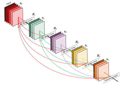
DenseNet
DenseNet models were proposed in the paper - “Densely Connected Convolutional Networks”. The authors of this paper used previously gained insights from approaches like ResNet. The DenseNet architecture incorporates all benefits of the ResNet architecture, alleviates the vanishing-gradient problem, which emerges in very deep networks, and, in addition, it improves the information handling. The proposed idea is that every output of a hidden layer is connected to the input of every following layer. How this looks like can be seen in the next figure. To put it simply, the information flow is realized in a feed-forward fashion. This allows the model or – to be more accurate – the output layer, to comprehend not only the information of one previous layer but all intermediate outputs of all the previous hidden layers. That means that the output of one of the first layers in the model, which in computer vision tasks are mostly focused on extracting edges or textures, is directly connected to the last layer. The same way as layers deeper in the network, which handle very complex patterns. This allows the last layer to combine simple features with complex patterns to conclude to a classification. In a general perspective, this architecture leads to feature propagation and feature reuse which allowed the model to outperform many other approaches. [Pytorch – DenseNet]
Evaluation Metrics
To monitor the training of our model as well as evaluate the model itself we tracked different metrics continuously to tensorboard:
Loss:
To see how the loss of our model performs during the training process we logged the average result of our loss function of a configurable number of training batches. Hence, we were able to stop a training process if we saw, the loss was not decreasing or even increasing or alternating.
distAn:
Therefore, we let our model during evaluation calculate the embeddings of the anchors and the positives and calculate the distance between these two vectors. We wanted to have these values above our predefined threshold of 10.
distAp:
Like distAn, but with anchor and negatives. We wanted to have this value very close to zero.
Accuracy:
We used to calculate an accuracy during the training process in the evaluation steps. If the distance between the anchor and the negative was smaller than the distance between the anchor and the negative the triplet was counted as hit.
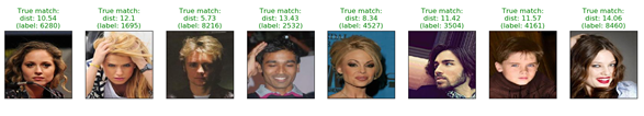
Sample Inferences:
To manually get an idea of the performance of the model, we let our model predict the id of a random image and logged the image with the prediction and the distance to its’ anchor to tensorboard. Furthermore, we logged some triplets with their distAp and distAn to tensorboard. Thus, we were able to inference some specific difficulties of our model.
Hyperparameter-Tuning
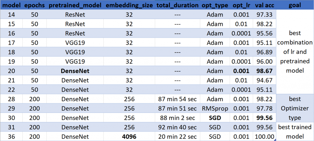
We started with three different pretrained models (DenseNet, VGG19, ResNet) and three different learning rates (0.01, 0.001, 0.0001). In two experiments with first 15 and then 50 epochs we tried to figure out, which combination of pretrained model and learning rate achieves the best results. In both the combination of the DenseNet with a learning rate of 0.001 performed best. In the next step we tried out three different optimizers. We experimented with the Adam optimizer, the RMSprop optimizer, and the stochastic gradient descent (SGD). Therefore, we used the predetermined combination of DenseNet with the learning rate of 0.001. For our case, the SGD optimizer worked best. In the last step we tried to optimize our model. First, we increased the dimension of our output-vector to 4096. Second, we doubled the number of features in the last three layers of our model. Third, we set the threshold to differentiate between a known and unknown person from 10 to 20 for the distance between the anchor and another image.
All of this led to a better validation accuracy. Furthermore, the training duration decreased significantly as we implemented a mechanism which stops the training when the total loss of a whole epoch is zero.
In the following table, you can find details about our trained models. The selected hyperparameters as well as the training accuracy of the experiment are marked bold.
Discussion of Results
Results Draw Conclusion to Features and Functionalities
We were very impressed by the accuracy even of the first attempts of our net. Not only of the accuracy and the loss, but even with the inference on the validation dataset. During training we logged several data to tensorboard to get a better understanding of what our model does during training.
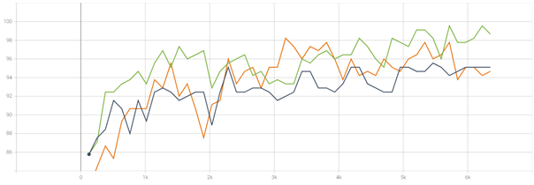
Figure 1 shows the accuracy during validation after each training epoch during hyperparameter training. One can see that the training with the learning rate of 0.001 performs best.
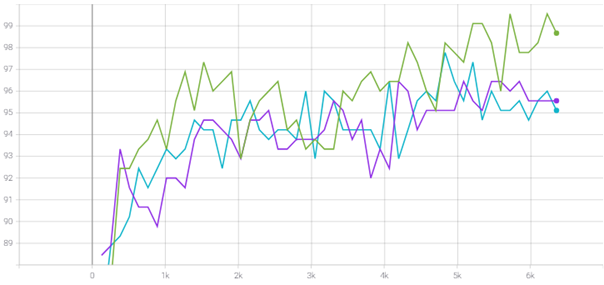
Figure 15 and 16 visualize our evaluation after each epoch.
In Figure 17 and 18 one can see the inference. The model gets an image of an arbitrary person and has to decide which person this is.
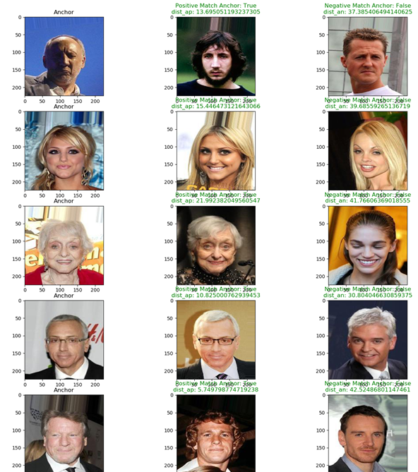
(Left: anchor, Center: positive, Right: negative)
Main Challenges
The main challenge was to deal with the huge amount of data. The preprocessing and the creation of the triplets for the whole dataset took several hours of computing time.
We tried several times to train our model with a bigger. But every time the loss during training decreased while it increased for the validation. Furthermore, the accuracy of the model decreased with the number of epochs and varied around 50% which is just as good as a dice. We still cannot explain why there is such a large difference in the behavior and performance of the model depending on the size of the dataset.
Ethical Aspects of Face Recognition
In the last decade machine learning has not only gained a lot of popularity, but also improved further to enable an even broader spectrum of application scenarios. This becomes particularly apparent for convolutional neural networks and their numerous variants, that can be applied to the tasks of image classification, image colorization, image reconstruction and inpainting, object detection, object segmentation and many more [17].
While this technological progress certainly facilitates numerous opportunities for innovative and high-performance system architectures, it is partially shadowed by increasing concerns about ethical aspects. Often, the applied implicit reasoning inside a complex machine learning model, for example a neural network, cannot be made transparent anymore to external requestors and – sometimes – not even to the people who created the model. This behavior marks the dawn of the call for explainable AI: Models should not exhibit ‘black box’ behavior, but the decisions should always remain transparent [18]. In this brief article we want to shed light on an ethical aspect of one of the most personal neural network applications: face recognition.
Face recognition has already made it into our everyday lives as a handy tool: Many people can already enjoy the convenience of unlocking their phones with a quick glance or appreciate the automatic tagging of people they love in their phones’ galleries. While these advantages face recognition can introduce to our lives are well advertised and praised, there are other face recognition applications currently used in practice, which have sparked a more serious discussion about their ethical implications. A recurring issue among face recognition systems is a supposedly racist tendency, which can discriminate entire social groups based on their ethnicity. Subsequently, we will briefly discuss two examples of such systems, depicting the impact they can introduce and examining a possible cause for their unjust reasoning.
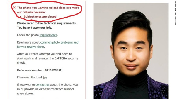
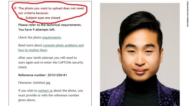
One such flawed application of face recognition technology is the automated passport creation system in New Zealand launched in 2016. One of the included tasks of this self-service process is to upload a personal biometric photo of the user’s face, in order to later identify them. But, as depicted by James Griffiths in his article on CNN, the system is unable to correctly detect the eyes of people of Asian descent as ‘open’ [19]. Repeatedly responding with an error message, the system is thereby blocking an entire ethnic group from finishing the passport creation process. This raises the ethical question of equality, as not all people can use this system equally well, or possibly, some people cannot use it at all.
The root causes of these kind of flaws in face recognition systems are often difficult to detect. While the system exhibits great performance, for example in terms of accuracy on the examined test set, it fails to perform similarly well in this real-world scenario. One possible cause of this phenomenon is a highly skewed dataset used to train the underlying model of the face recognition system. This problem is called a biased dataset and can severely impact the performance of a machine learning system [20]. In the above case, the dataset and thus the model are biased towards e.g. Caucasian faces. As the model has (almost) only seen faces of people of Caucasian, it has no point of reference to accurately perform on faces of people of Asian descent. Thus, the model cannot comprehend all the variety of faces it can be exposed to in practice.
Another exemplary system, with even more severe implication to its ‘users’, can be found in a pilot experiment conducted by U.S. justice and rehabilitation authorities. The developed system aims to predict the risk of a convict to commit additional crimes in the future. By outputting a ‘risk score’ it can potentially aid the authorities to decide on measures for surveilling and restricting individuals. But, as shown in an extensive ProPublica article, this system exhibits a fundamental racist tendency against people of African American origin [21]. By assigning consistently higher risk scores to their ethnic group, this system – with its incisive repercussions – again raises strong concerns for equality.
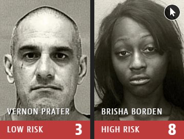
The underlying bias problem introduced to this model is of contrary origin: The discriminated group appeared disproportionally often in the training data. Thus, the system concluded a general rule, basing high risk scores to a large extent on skin color.
Besides this issue of ill-balanced datasets, there exist other unconscious racial biases in face recognition systems that can be difficult to detect and prevent [22]. If the triumphal procession of face recognition and other machine learning techniques shall continue in a throughout positive manner, these inadvertent flaws need to be reliably detected and resolved early on. Else, the resulting unjust implications can persist until they are exposed during productive use, resulting in severe implications for people exposed to them, as depicted in the two above examples.
Conclusion and Outlook
In this last chapter we want to draw a conclusion of the past three months and provide an outlook for possible use cases of our work. Furthermore, we are classifying the topic of face recognition with regard to the state of the art.
On a personal level, all of us could extend their personal skills and acquire new knowledge in various domains through this project. None of us was familiar beyond the basics of face recognition and its difficulties. The same applies to One-Shot-Learning. Even though all of us got experience in Python and Machine Learning, none of us ever worked with PyTorch or extensively used tensorboard to track the neural network’s performance. By using Streamlit we got to know a good tool to build presentable prototypes.
The speech about the moral aspects of face recognition by the IBM contributors (shoutout to Sebastian), in combination with the self-study of this topic, created an awareness for the responsibility that is related to face recognition technologies. It brings both benefits and disadvantages and should be treated with caution.
From the technical perspective, face recognition as we implemented it is already highly sophisticated. With an accuracy of above 99% it leaves only very little scope for improvement. We therefore see more opportunities in the research fields of 3D face recognition, make-up face recognition and prevention of adversarial attacks.
Overall, we enjoyed working on the topic of face recognition and are grateful for the provided technical environment by TUM and IBM. We improved in both the theory and the practical implementation of face recognition approaches, while also strengthening our communicational and organizational skills in our team. We can recommend this practical course to future students that are interested in an interesting yet challenging machine learning project.
Bibliography / References
[1] M. Wang and W. Deng, “Deep Face Recognition: A Survey.”
[2] Y. Taigman, M. Y. Marc’, A. Ranzato, and L. Wolf, “DeepFace: Closing the Gap to Human-Level Performance in Face Verification.”
[3] O. M. Parkhi, A. Vedaldi, and A. Zisserman, “Deep Face Recognition.”
[4] F. Schroff and J. Philbin, “FaceNet: A Unified Embedding for Face Recognition and Clustering.”
[5] K. Simonyan and A. Zisserman, “VERY DEEP CONVOLUTIONAL NETWORKS FOR LARGE-SCALE IMAGE RECOGNITION,” 2015.
[6] S. Sengupta, J.-C. Chen, C. Castillo, V. M. Patel, R. Chellappa, and D. W. Jacobs, “Frontal to Profile Face Verification in the Wild.”
[7] T. Zheng, W. Deng, and J. Hu, “Age Estimation Guided Convolutional Neural Network for Age-Invariant Face Recognition.”
[8] V. Kushwaha, M. Singh, R. Singh, M. Vatsa, N. Ratha, and R. Chellappa, “Disguised Faces in the Wild.”
[9] T. Ahonen, A. Hadid, and M. Pietikäinen, “Face recognition with local binary patterns,” Lect. Notes Comput. Sci. (including Subser. Lect. Notes Artif. Intell. Lect. Notes Bioinformatics), vol. 3021, pp. 469–481, 2004, doi: 10.1007/978-3-540-24670-1_36.
[10] D. Chen, X. Cao, F. Wen, and J. Sun, “Blessing of dimensionality: High-dimensional feature and its efficient compression for face verification,” in Proceedings of the IEEE Computer Society Conference on Computer Vision and Pattern Recognition, 2013, pp. 3025–3032, doi: 10.1109/CVPR.2013.389.
[11] W. Deng, J. Hu, and J. Guo, “Compressive Binary Patterns: Designing a Robust Binary Face Descriptor with Random-Field Eigenfilters,” IEEE Trans. Pattern Anal. Mach. Intell., vol. 41, no. 3, pp. 758–767, Mar. 2019, doi: 10.1109/TPAMI.2018.2800008.
[12] Y. Taigman, M. Y. Marc’, A. Ranzato, and L. Wolf, “DeepFace: Closing the Gap to Human-Level Performance in Face Verification.” Accessed: Jan. 18, 2021. [Online]. Available: https://www.cv-foundation.org/openaccess/content_cvpr_2014/papers/Taigman_DeepFace_Closing_the_2014_CVPR_paper.pdf.
[13] F. Schroff and J. Philbin, “FaceNet: A Unified Embedding for Face Recognition and Clustering.” Accessed: Jan. 19, 2021. [Online]. Available: https://www.cv-foundation.org/openaccess/content_cvpr_2015/papers/Schroff_FaceNet_A_Unified_2015_CVPR_paper.pdf.
[14] O. M. Parkhi, A. Vedaldi, and A. Zisserman, “Deep Face Recognition.” Accessed: Jan. 19, 2021. [Online]. Available: https://ora.ox.ac.uk/objects/uuid:a5f2e93f-2768-45bb-8508-74747f85cad1/download_file?file_format=pdf&safe_filename=parkhi15.pdf&type_of_work=Conference+item.
[15] Q. Cao, L. Shen, W. Xie, O. M. Parkhi, and A. Zisserman, “VGGFace2: A dataset for recognising faces across pose and age,” Proc. - 13th IEEE Int. Conf. Autom. Face Gesture Recognition, FG 2018, pp. 67–74, 2018, doi: 10.1109/FG.2018.00020.
[16] Z. Liu, P. Luo, X. Wang, and X. Tang, “Deep learning face attributes in the wild,” Proc. IEEE Int. Conf. Comput. Vis., vol. 2015 Inter, no. February, pp. 3730–3738, 2015, doi: 10.1109/ICCV.2015.425.
[17] A. I. Khan and S. Al-Habsi, “Machine Learning in Computer Vision,” Procedia Comput. Sci., vol. 167, no. 2019, pp. 1444–1451, 2020, doi: 10.1016/j.procs.2020.03.355.
[18] A. Adadi and M. Berrada, “Peeking Inside the Black-Box: A Survey on Explainable Artificial Intelligence (XAI),” IEEE Access, vol. 6, pp. 52138–52160, Sep. 2018, doi: 10.1109/ACCESS.2018.2870052.
[19] J. Griffiths, “New Zealand passport robot thinks this Asian man’s eyes are closed,” Cnn, 2016. https://edition.cnn.com/2016/12/07/asia/new-zealand-passport-robot-asian-trnd/index.html (accessed Jan. 21, 2021).
[20] T. Tommasi, N. Patricia, B. Caputo, and T. Tuytelaars, “A deeper look at dataset bias,” in Advances in Computer Vision and Pattern Recognition, no. 9783319583464, Springer London, 2017, pp. 37–55.
[21] L. Kirchner, S. Mattu, J. Larson, and J. Angwin, “Machine Bias,” Propublica, pp. 1–26, 2016, Accessed: Jan. 21, 2021. [Online]. Available: https://www.propublica.org/article/machine-bias-risk-assessments-in-criminal-sentencing.
[22] J. G. Cavazos, P. Jonathon Phillips, C. D. Castillo, and A. J. O’Toole, “Accuracy comparison across face recognition algorithms: Where are we on measuring race bias?,” arXiv. arXiv, Dec. 16, 2019, doi: 10.1109/tbiom.2020.3027269.
Appendix
Appendix: